PackedSelection in Coffea 2023
In coffea, PackedSelection is a class that can store several boolean arrays in a memory-efficient manner and evaluate arbitrary combinations of boolean requirements in an CPU-efficient way. Supported inputs include 1D numpy or awkward arrays and it has built-in functionalities to form analysis in signal and control regions, and to implement cutflow or “N-1” plots.
Although coffea 2023 should be used in delayed mode (using dask-awkward), we will first present these functionalities eagerly (like in coffea 0.7) to showcase this better. Let’s first read a sample file of 40 Drell-Yan events to demonstrate the utilities using our NanoAODSchema as our schema.
[1]:
import awkward as ak
import numpy as np
from coffea.nanoevents import NanoEventsFactory, NanoAODSchema
from matplotlib import pyplot as plt


events = NanoEventsFactory.from_root(
    {"../tests/samples/nano_dy.root": "Events"},
    metadata={"dataset": "nano_dy"},
    schemaclass=NanoAODSchema,
    permit_dask=False,
).events()

events
/Users/iason/fun/coffea_dev/coffea/binder/coffea/nanoevents/schemas/nanoaod.py:215: RuntimeWarning: Missing cross-reference index for FatJet_genJetAK8Idx => GenJetAK8
  warnings.warn(
[1]:
[{FsrPhoton: [], Electron: [], SoftActivityJetHT5: 63.5, RawMET: {...}, ...},
 {FsrPhoton: [], Electron: [{...}], SoftActivityJetHT5: 64, RawMET: {...}, ...},
 {FsrPhoton: [], Electron: [Electron, Electron], SoftActivityJetHT5: 130, ...},
 {FsrPhoton: [], Electron: [Electron, Electron], SoftActivityJetHT5: 25.8, ...},
 {FsrPhoton: [], Electron: [], SoftActivityJetHT5: 172, RawMET: {...}, ...},
 {FsrPhoton: [], Electron: [{...}], SoftActivityJetHT5: 54.4, RawMET: ..., ...},
 {FsrPhoton: [], Electron: [{...}], SoftActivityJetHT5: 96.2, RawMET: ..., ...},
 {FsrPhoton: [], Electron: [], SoftActivityJetHT5: 19, RawMET: {...}, ...},
 {FsrPhoton: [], Electron: [], SoftActivityJetHT5: 9.36, RawMET: {...}, ...},
 {FsrPhoton: [], Electron: [{...}], SoftActivityJetHT5: 115, RawMET: ..., ...},
 ...,
 {FsrPhoton: [], Electron: [{...}], SoftActivityJetHT5: 49.6, RawMET: ..., ...},
 {FsrPhoton: [], Electron: [], SoftActivityJetHT5: 14.7, RawMET: {...}, ...},
 {FsrPhoton: [], Electron: [{...}], SoftActivityJetHT5: 22.1, RawMET: ..., ...},
 {FsrPhoton: [], Electron: [], SoftActivityJetHT5: 33.9, RawMET: {...}, ...},
 {FsrPhoton: [], Electron: [{...}], SoftActivityJetHT5: 16.2, RawMET: ..., ...},
 {FsrPhoton: [], Electron: [], SoftActivityJetHT5: 28.4, RawMET: {...}, ...},
 {FsrPhoton: [], Electron: [{...}], SoftActivityJetHT5: 16.1, RawMET: ..., ...},
 {FsrPhoton: [], Electron: [], SoftActivityJetHT5: 28.5, RawMET: {...}, ...},
 {FsrPhoton: [], Electron: [], SoftActivityJetHT5: 7, RawMET: {...}, ...}]
--------------------------------------------------------------------------------
type: 40 * event
Now let’s import PackedSelection, and create an instance of it.
[2]:
from coffea.analysis_tools import PackedSelection

selection = PackedSelection()
We can create a boolean mask and add this to our selection by using the add method. This adds the following “cut” to our selection and names it “twoElectron”.
[3]:
selection.add("twoElectron", ak.num(events.Electron) == 2)
We’ve added one “cut” to our selection. Now let’s add a couple more.
[4]:
selection.add("eleOppSign", ak.sum(events.Electron.charge, axis=1) == 0)
selection.add("noElectron", ak.num(events.Electron) == 0)
To avoid repeating calling add multiple times, we can just use the add_multiple method which does just that.
[5]:
selection.add_multiple(
    {
        "twoMuon": ak.num(events.Muon) == 2,
        "muOppSign": ak.sum(events.Muon.charge, axis=1) == 0,
        "noMuon": ak.num(events.Muon) == 0,
        "leadPt20": ak.any(events.Electron.pt >= 20.0, axis=1)
        | ak.any(events.Muon.pt >= 20.0, axis=1),
    }
)
By viewing the PackedSelection instance, one can see the names of the added selections, whether it is operating in delayed mode or not, the number of added selections and the maximum supported number of selections.
[6]:
print(selection)
PackedSelection(selections=('twoElectron', 'eleOppSign', 'noElectron', 'twoMuon', 'muOppSign', 'noMuon', 'leadPt20'), delayed_mode=False, items=7, maxitems=32)
To evaluate a boolean mask (e.g. to filter events) we can use the selection.all(*names) function, which will compute the logical AND of all listed boolean selections.
[7]:
selection.all("twoElectron", "noMuon", "leadPt20")
[7]:
array([False, False,  True, False, False, False, False, False, False,
       False, False, False, False, False, False, False, False, False,
       False, False,  True,  True, False, False, False, False, False,
       False, False, False, False, False, False, False, False, False,
       False, False, False, False])
We can also be more specific and require that a specific set of selections have a given value (with the unspecified ones allowed to be either true or false) using selection.require.
[8]:
selection.require(twoElectron=True, noMuon=True, eleOppSign=False)
[8]:
array([False, False, False,  True, False, False, False, False, False,
       False, False, False, False, False, False, False, False, False,
       False, False, False, False, False, False, False, False, False,
       False, False, False, False, False, False, False, False, False,
       False, False, False, False])
There exist also the allfalse and any methods where the first one is the opposite of all and the second one is a logical OR between all listed boolean selections.
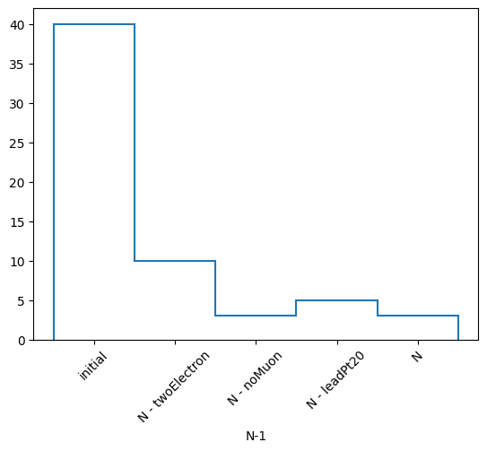
Using PackedSelection, we are now able to perform an N-1 style selection using the nminusone(*names) method. This will perform an N-1 style selection by using as “N” the provided names and will exclude each named cut one at a time in order. In the end it will also peform a selection using all N cuts.
[9]:
nminusone = selection.nminusone("twoElectron", "noMuon", "leadPt20")
nminusone
[9]:
NminusOne(selections=('twoElectron', 'noMuon', 'leadPt20'))
This returns an NminusOne object which has the following methods: result(), print(), yieldhist(), to_npz() and plot_vars()
Let’s look at the results of the N-1 selection.
[10]:
res = nminusone.result()
print(type(res), res._fields)
<class 'coffea.analysis_tools.NminusOneResult'> ('labels', 'nev', 'masks')
This is just a namedtuple with the attributes labels, nev and masks. So we can say:
[11]:
labels, nev, masks = res
labels, nev, masks
[11]:
(['initial', 'N - twoElectron', 'N - noMuon', 'N - leadPt20', 'N'],
 [40, 10, 3, 5, 3],
 [array([False,  True,  True, False, False, False, False, False, False,
          True, False, False, False, False, False,  True,  True, False,
         False, False,  True,  True, False, False, False, False, False,
          True, False,  True, False, False, False,  True, False, False,
         False, False, False, False]),
  array([False, False,  True, False, False, False, False, False, False,
         False, False, False, False, False, False, False, False, False,
         False, False,  True,  True, False, False, False, False, False,
         False, False, False, False, False, False, False, False, False,
         False, False, False, False]),
  array([False, False,  True,  True, False, False, False, False, False,
         False, False, False, False, False, False, False, False, False,
          True, False,  True,  True, False, False, False, False, False,
         False, False, False, False, False, False, False, False, False,
         False, False, False, False]),
  array([False, False,  True, False, False, False, False, False, False,
         False, False, False, False, False, False, False, False, False,
         False, False,  True,  True, False, False, False, False, False,
         False, False, False, False, False, False, False, False, False,
         False, False, False, False])])
labels is a list of labels of each mask that is applied, nev is a list of the number of events that survive each mask, and masks is a list of boolean masks (arrays) of which events survive each selection. You can also choose to print the statistics of your N-1 selection in a similar fashion to RDataFrame.
[12]:
nminusone.print()
N-1 selection stats:
Ignoring twoElectron         : pass = 10                                  all = 40                                  -- eff = 25.0 %
Ignoring noMuon              : pass = 3                                   all = 40                                  -- eff = 7.5 %
Ignoring leadPt20            : pass = 5                                   all = 40                                  -- eff = 12.5 %
All cuts                     : pass = 3                                   all = 40                                  -- eff = 7.5 %
Or get a histogram of your total event yields. This just returns a hist.Hist object and we can plot it with its backends to mplhep.
[13]:
h, labels = nminusone.yieldhist()
h.plot1d()
plt.xticks(plt.gca().get_xticks(), labels, rotation=45)
plt.show()

You can also save the results of the N-1 selection to a .npz file for later use.
[14]:
nminusone.to_npz("nminusone_results.npz")

with np.load("nminusone_results.npz") as f:
    for i in f.files:
        print(f"{i}: {f[i]}")
labels: ['initial' 'N - twoElectron' 'N - noMuon' 'N - leadPt20' 'N']
nev: [40 10  3  5  3]
masks: [[False  True  True False False False False False False  True False False
  False False False  True  True False False False  True  True False False
  False False False  True False  True False False False  True False False
  False False False False]
 [False False  True False False False False False False False False False
  False False False False False False False False  True  True False False
  False False False False False False False False False False False False
  False False False False]
 [False False  True  True False False False False False False False False
  False False False False False False  True False  True  True False False
  False False False False False False False False False False False False
  False False False False]
 [False False  True False False False False False False False False False
  False False False False False False False False  True  True False False
  False False False False False False False False False False False False
  False False False False]]
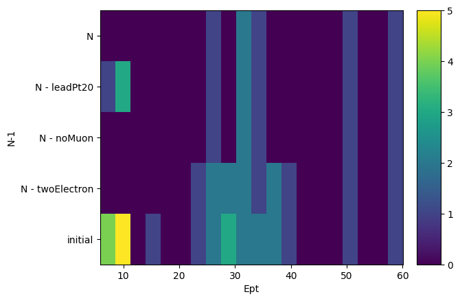
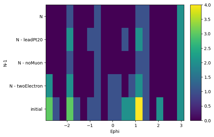
Finally, we can ask from this object to create histograms of different variables, masking them with our N-1 selection. What it will output is a list of histograms, one for each requested variable, where the x-axis is the distribution of the variable, and the y-axis is the mask that was applied. It is essentially slices of how the variable distribution evolves as each N-1 or N selection is applied. It does also return a list of labels of the masks to keep track.
Note that the variables are parsed using a dictonary of name: array pairs and that the arrays will of course be flattened to be histogrammed.
[15]:
hs, labels = nminusone.plot_vars(
    {"Ept": events.Electron.pt, "Ephi": events.Electron.phi}
)
hs, labels
[15]:
([Hist(
    Regular(20, 5.81891, 60.0685, name='Ept'),
    Integer(0, 5, name='N-1'),
    storage=Double()) # Sum: 60.0,
  Hist(
    Regular(20, -2.93115, 3.11865, name='Ephi'),
    Integer(0, 5, name='N-1'),
    storage=Double()) # Sum: 60.0],
 ['initial', 'N - twoElectron', 'N - noMuon', 'N - leadPt20', 'N'])
And we can actually plot those histograms using again the mplhep backend.
[16]:
for h in hs:
    h.plot2d()
    plt.yticks(plt.gca().get_yticks(), labels, rotation=0)
    plt.show()
You can slice these histograms to view and plot the 1D histogram at each step of the selection. For example, if we want the \(P_T\) of the electrons at the final step (index 4) of the selection, we can do the following.
[17]:
hs[0][:, 4].plot1d(yerr=0)
plt.yscale("log")
plt.show()
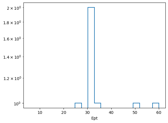
Because this automatic bining doesn’t look great, for \(P_T\) at least, the user has the ability to customize the axes or pass in their own axes objects.
[18]:
help(nminusone.plot_vars)
Help on method plot_vars in module coffea.analysis_tools:

plot_vars(vars, axes=None, bins=None, start=None, stop=None, edges=None, transform=None) method of coffea.analysis_tools.NminusOne instance
    Plot the histograms of variables for each step of the N-1 selection

    Parameters
    ----------
        vars : dict
            A dictionary in the form ``{name: array}`` where ``name`` is the name of the variable,
            and ``array`` is the corresponding array of values.
            The arrays must be the same length as each mask of the N-1 selection.
        axes : list of hist.axis objects, optional
            The axes objects to histogram the variables on. This will override all the following arguments that define axes.
            Must be the same length as ``vars``.
        bins : iterable of integers or Nones, optional
            The number of bins for each variable histogram. If not specified, it defaults to 20.
            Must be the same length as ``vars``.
        start : iterable of floats or integers or Nones, optional
            The lower edge of the first bin for each variable histogram. If not specified, it defaults to the minimum value of the variable array.
            Must be the same length as ``vars``.
        stop : iterable of floats or integers or Nones, optional
            The upper edge of the last bin for each variable histogram. If not specified, it defaults to the maximum value of the variable array.
            Must be the same length as ``vars``.
        edges : list of iterables of floats or integers, optional
            The bin edges for each variable histogram. This overrides ``bins``, ``start``, and ``stop`` if specified.
            Must be the same length as ``vars``.
        transform : iterable of hist.axis.transform objects or Nones, optional
            The transforms to apply to each variable histogram axis. If not specified, it defaults to None.
            Must be the same length as ``vars``.

    Returns
    -------
        hists : list of hist.Hist or hist.dask.Hist objects
            A list of 2D histograms of the variables for each step of the N-1 selection.
            The first axis is the variable, the second axis is the N-1 selection step.
        labels : list of strings
            The bin labels of y axis of the histogram.
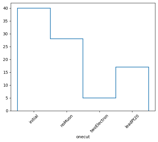
Cutflow is implemented in a similar manner to the N-1 selection. We just have to use the cutflow(*names) function which will return a Cutflow object
[19]:
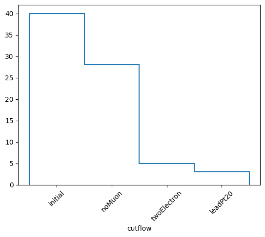
cutflow = selection.cutflow("noMuon", "twoElectron", "leadPt20")
cutflow
[19]:
Cutflow(selections=('noMuon', 'twoElectron', 'leadPt20'))
The methods of this object are similar to the NminusOne object. The only difference is that now we seperate things in either “onecut” or “cutflow”. “onecut” represents results where each cut is applied alone, while “cutflow” represents results where the cuts are applied cumulatively in order.
[20]:
res = cutflow.result()
print(type(res), res._fields)
labels, nevonecut, nevcutflow, masksonecut, maskscutflow = res
labels, nevonecut, nevcutflow, masksonecut, maskscutflow
<class 'coffea.analysis_tools.CutflowResult'> ('labels', 'nevonecut', 'nevcutflow', 'masksonecut', 'maskscutflow')
[20]:
(['initial', 'noMuon', 'twoElectron', 'leadPt20'],
 [40, 28, 5, 17],
 [40, 28, 5, 3],
 [array([ True,  True,  True,  True, False, False, False,  True,  True,
          True, False,  True,  True,  True, False,  True,  True,  True,
          True,  True,  True,  True,  True, False, False,  True, False,
          True, False,  True, False, False,  True,  True, False,  True,
          True,  True,  True,  True]),
  array([False, False,  True,  True, False, False, False, False, False,
         False, False, False, False, False, False, False, False, False,
          True, False,  True,  True, False, False, False, False, False,
         False, False, False, False, False, False, False, False, False,
         False, False, False, False]),
  array([False,  True,  True, False,  True,  True,  True, False, False,
          True, False, False, False, False, False,  True,  True, False,
         False, False,  True,  True, False,  True,  True, False,  True,
          True, False,  True, False,  True, False,  True, False, False,
         False, False, False, False])],
 [array([ True,  True,  True,  True, False, False, False,  True,  True,
          True, False,  True,  True,  True, False,  True,  True,  True,
          True,  True,  True,  True,  True, False, False,  True, False,
          True, False,  True, False, False,  True,  True, False,  True,
          True,  True,  True,  True]),
  array([False, False,  True,  True, False, False, False, False, False,
         False, False, False, False, False, False, False, False, False,
          True, False,  True,  True, False, False, False, False, False,
         False, False, False, False, False, False, False, False, False,
         False, False, False, False]),
  array([False, False,  True, False, False, False, False, False, False,
         False, False, False, False, False, False, False, False, False,
         False, False,  True,  True, False, False, False, False, False,
         False, False, False, False, False, False, False, False, False,
         False, False, False, False])])
As you can see, again we have the same labels, nev and masks only now we have two “versions” of them since they’ve been split into “onecut” and “cutflow”. You can again print the statistics of the cutflow exactly like RDataFrame.
[21]:
cutflow.print()
Cutflow stats:
Cut noMuon              : pass = 28                                  cumulative pass = 28                                  all = 40                                  --  eff = 70.0 %                -- cumulative eff = 70.0 %
Cut twoElectron         : pass = 5                                   cumulative pass = 5                                   all = 40                                  --  eff = 12.5 %                -- cumulative eff = 12.5 %
Cut leadPt20            : pass = 17                                  cumulative pass = 3                                   all = 40                                  --  eff = 42.5 %                -- cumulative eff = 7.5 %
Again, you can extract yield hists, only now there are two of them.
[22]:
honecut, hcutflow, labels = cutflow.yieldhist()

honecut.plot1d(yerr=0)
plt.xticks(plt.gca().get_xticks(), labels, rotation=45)
plt.show()

hcutflow.plot1d(yerr=0)
plt.xticks(plt.gca().get_xticks(), labels, rotation=45)
plt.show()
Saving to .npz files is again there.
[23]:
cutflow.to_npz("cutflow_results.npz")

with np.load("cutflow_results.npz") as f:
    for i in f.files:
        print(f"{i}: {f[i]}")
labels: ['initial' 'noMuon' 'twoElectron' 'leadPt20']
nevonecut: [40 28  5 17]
nevcutflow: [40 28  5  3]
masksonecut: [[ True  True  True  True False False False  True  True  True False  True
   True  True False  True  True  True  True  True  True  True  True False
  False  True False  True False  True False False  True  True False  True
   True  True  True  True]
 [False False  True  True False False False False False False False False
  False False False False False False  True False  True  True False False
  False False False False False False False False False False False False
  False False False False]
 [False  True  True False  True  True  True False False  True False False
  False False False  True  True False False False  True  True False  True
   True False  True  True False  True False  True False  True False False
  False False False False]]
maskscutflow: [[ True  True  True  True False False False  True  True  True False  True
   True  True False  True  True  True  True  True  True  True  True False
  False  True False  True False  True False False  True  True False  True
   True  True  True  True]
 [False False  True  True False False False False False False False False
  False False False False False False  True False  True  True False False
  False False False False False False False False False False False False
  False False False False]
 [False False  True False False False False False False False False False
  False False False False False False False False  True  True False False
  False False False False False False False False False False False False
  False False False False]]
And finally, plot_vars is also there with the same axes customizability while now it returns two lists of histograms, one for “onecut” and one for “cutflow”. Those can of course be plotted in a similar fashion.
[24]:
h1, h2, labels = cutflow.plot_vars(
    {"ept": events.Electron.pt, "ephi": events.Electron.phi}
)
h1, h2, labels
[24]:
([Hist(
    Regular(20, 5.81891, 60.0685, name='ept'),
    Integer(0, 4, name='onecut'),
    storage=Double()) # Sum: 73.0,
  Hist(
    Regular(20, -2.93115, 3.11865, name='ephi'),
    Integer(0, 4, name='onecut'),
    storage=Double()) # Sum: 73.0],
 [Hist(
    Regular(20, 5.81891, 60.0685, name='ept'),
    Integer(0, 4, name='cutflow'),
    storage=Double()) # Sum: 63.0,
  Hist(
    Regular(20, -2.93115, 3.11865, name='ephi'),
    Integer(0, 4, name='cutflow'),
    storage=Double()) # Sum: 63.0],
 ['initial', 'noMuon', 'twoElectron', 'leadPt20'])
Now, in coffea 2023, everything happens in a delayed fashion. Therefore, PackedSelection can also operate in delayed or lazy mode and fully support dask_awkward arrays. Use is still the same, but everything now is a delayed dask type object which can be computed whenever the user wants to. This can be done by either calling .compute() on the object or dask.compute(*things).
PackedSelection can be initialized to operate in delayed mode by adding a delayed dask_awkward array for the first time instead of a materialized numpy or awkward one. I would like to note that we only support delayed dask_awkward arrays and not dask.array arrays. Please convert your dask arrays to dask_awkward via dask_awkward.from_dask_array(array). I would also like to note that you cannot mix materialized and delayed arrays in the same PackedSelection.
Let’s now read the same events using dask and perform the exact same things.
[25]:
import dask
import dask_awkward as dak

dakevents = NanoEventsFactory.from_root(
    {"../tests/samples/nano_dy.root": "Events"},
    metadata={"dataset": "nano_dy"},
    schemaclass=NanoAODSchema,
    permit_dask=True,
).events()

dakevents
/Users/iason/fun/coffea_dev/coffea/binder/coffea/nanoevents/schemas/nanoaod.py:215: RuntimeWarning: Missing cross-reference index for FatJet_genJetAK8Idx => GenJetAK8
  warnings.warn(
[25]:
dask.awkward<from-uproot, npartitions=1>
Now dakevents is a delayed dask_awkward version of our events and if we compute it we get our normal events.
[26]:
dakevents.compute()
[26]:
[{FsrPhoton: [], Electron: [], SoftActivityJetHT5: 63.5, RawMET: {...}, ...},
 {FsrPhoton: [], Electron: [{...}], SoftActivityJetHT5: 64, RawMET: {...}, ...},
 {FsrPhoton: [], Electron: [Electron, Electron], SoftActivityJetHT5: 130, ...},
 {FsrPhoton: [], Electron: [Electron, Electron], SoftActivityJetHT5: 25.8, ...},
 {FsrPhoton: [], Electron: [], SoftActivityJetHT5: 172, RawMET: {...}, ...},
 {FsrPhoton: [], Electron: [{...}], SoftActivityJetHT5: 54.4, RawMET: ..., ...},
 {FsrPhoton: [], Electron: [{...}], SoftActivityJetHT5: 96.2, RawMET: ..., ...},
 {FsrPhoton: [], Electron: [], SoftActivityJetHT5: 19, RawMET: {...}, ...},
 {FsrPhoton: [], Electron: [], SoftActivityJetHT5: 9.36, RawMET: {...}, ...},
 {FsrPhoton: [], Electron: [{...}], SoftActivityJetHT5: 115, RawMET: ..., ...},
 ...,
 {FsrPhoton: [], Electron: [{...}], SoftActivityJetHT5: 49.6, RawMET: ..., ...},
 {FsrPhoton: [], Electron: [], SoftActivityJetHT5: 14.7, RawMET: {...}, ...},
 {FsrPhoton: [], Electron: [{...}], SoftActivityJetHT5: 22.1, RawMET: ..., ...},
 {FsrPhoton: [], Electron: [], SoftActivityJetHT5: 33.9, RawMET: {...}, ...},
 {FsrPhoton: [], Electron: [{...}], SoftActivityJetHT5: 16.2, RawMET: ..., ...},
 {FsrPhoton: [], Electron: [], SoftActivityJetHT5: 28.4, RawMET: {...}, ...},
 {FsrPhoton: [], Electron: [{...}], SoftActivityJetHT5: 16.1, RawMET: ..., ...},
 {FsrPhoton: [], Electron: [], SoftActivityJetHT5: 28.5, RawMET: {...}, ...},
 {FsrPhoton: [], Electron: [], SoftActivityJetHT5: 7, RawMET: {...}, ...}]
--------------------------------------------------------------------------------
type: 40 * event
Now we have to use dask_awkward instead of awkward and dakevents instead of events to do the same things. Let’s add the same (now delayed) arrays to PackedSelection.
[27]:
selection = PackedSelection()

selection.add_multiple(
    {
        "twoElectron": dak.num(dakevents.Electron) == 2,
        "eleOppSign": dak.sum(dakevents.Electron.charge, axis=1) == 0,
        "noElectron": dak.num(dakevents.Electron) == 0,
        "twoMuon": dak.num(dakevents.Muon) == 2,
        "muOppSign": dak.sum(dakevents.Muon.charge, axis=1) == 0,
        "noMuon": dak.num(dakevents.Muon) == 0,
        "leadPt20": dak.any(dakevents.Electron.pt >= 20.0, axis=1)
        | dak.any(dakevents.Muon.pt >= 20.0, axis=1),
    }
)

print(selection)
PackedSelection(selections=('twoElectron', 'eleOppSign', 'noElectron', 'twoMuon', 'muOppSign', 'noMuon', 'leadPt20'), delayed_mode=True, items=7, maxitems=32)
Now, the same functions will return dask_awkward objects that have to be computed.
[28]:
selection.all("twoElectron", "noMuon", "leadPt20")
[28]:
dask.awkward<equal, npartitions=1>
When computing those arrays we should get the same arrays that we got when operating in eager mode.
[29]:
print(selection.all("twoElectron", "noMuon", "leadPt20").compute())
print(selection.require(twoElectron=True, noMuon=True, eleOppSign=False).compute())
[False, False, True, False, False, ..., False, False, False, False, False]
[False, False, False, True, False, ..., False, False, False, False, False]
Now, N-1 and cutflow will just return only delayed objects that must be computed.
[30]:
nminusone = selection.nminusone("twoElectron", "noMuon", "leadPt20")
nminusone
[30]:
NminusOne(selections=('twoElectron', 'noMuon', 'leadPt20'))
It is again an NminusOne object which has the same methods.
Let’s look at the results of the N-1 selection in the same way
[31]:
labels, nev, masks = nminusone.result()
labels, nev, masks
[31]:
(['initial', 'N - twoElectron', 'N - noMuon', 'N - leadPt20', 'N'],
 [dask.awkward<count, type=Scalar, dtype=int64>,
  dask.awkward<sum, type=Scalar, dtype=int64>,
  dask.awkward<sum, type=Scalar, dtype=int64>,
  dask.awkward<sum, type=Scalar, dtype=int64>,
  dask.awkward<sum, type=Scalar, dtype=int64>],
 [dask.awkward<equal, npartitions=1>,
  dask.awkward<equal, npartitions=1>,
  dask.awkward<equal, npartitions=1>,
  dask.awkward<equal, npartitions=1>])
Now however, you can see that everything is a dask awkward object (apart from the labels of course). If we compute them we should get the same things as before and indeed we do:
[32]:
dask.compute(*nev), dask.compute(*masks)
[32]:
((40, 10, 3, 5, 3),
 (<Array [False, True, True, False, ..., False, False, False] type='40 * bool'>,
  <Array [False, False, True, False, ..., False, False, False] type='40 * bool'>,
  <Array [False, False, True, True, ..., False, False, False] type='40 * bool'>,
  <Array [False, False, True, False, ..., False, False, False] type='40 * bool'>))
We can again print the statistics, however for this to happen, the object must of course compute the delayed nev list.
[33]:
nminusone.print()
N-1 selection stats:
Ignoring twoElectron         : pass = 10                                  all = 40                                  -- eff = 25.0 %
Ignoring noMuon              : pass = 3                                   all = 40                                  -- eff = 7.5 %
Ignoring leadPt20            : pass = 5                                   all = 40                                  -- eff = 12.5 %
All cuts                     : pass = 3                                   all = 40                                  -- eff = 7.5 %
And now if we call result() again, the nev list is materialized.
[34]:
nminusone.result().nev
[34]:
[40, 10, 3, 5, 3]
Again the histogram of your total event yields works. This time it is returns a hist.dask.Hist object.
[35]:
h, labels = nminusone.yieldhist()
h
[35]:
Double() Σ=0.0
It appears empty because it hasn’t been computed yet. Let’s do that.
[36]:
h.compute()
[36]:
Double() Σ=61.0
Notice that this doesn’t happen in place as h is still not computed.
[37]:
h
[37]:
Double() Σ=0.0
We can again plot this histogram but we have to call plot on the computed one, otherwise it will just be empty.
[38]:
h.compute().plot1d()
plt.xticks(plt.gca().get_xticks(), labels, rotation=45)
plt.show()
And we got exactly the same thing. Saving to .npz files is still possible but the delayed arrays will be naturally materalized while saving.
[39]:
nminusone.to_npz("nminusone_results.npz")

with np.load("nminusone_results.npz") as f:
    for i in f.files:
        print(f"{i}: {f[i]}")
labels: ['initial' 'N - twoElectron' 'N - noMuon' 'N - leadPt20' 'N']
nev: [40 10  3  5  3]
masks: [[False  True  True False False False False False False  True False False
  False False False  True  True False False False  True  True False False
  False False False  True False  True False False False  True False False
  False False False False]
 [False False  True False False False False False False False False False
  False False False False False False False False  True  True False False
  False False False False False False False False False False False False
  False False False False]
 [False False  True  True False False False False False False False False
  False False False False False False  True False  True  True False False
  False False False False False False False False False False False False
  False False False False]
 [False False  True False False False False False False False False False
  False False False False False False False False  True  True False False
  False False False False False False False False False False False False
  False False False False]]
Same logic applies to the plot_vars function. Remember to use dakevents now and not events.
[40]:
hs, labels = nminusone.plot_vars(
    {"Ept": dakevents.Electron.pt, "Ephi": dakevents.Electron.phi}
)
Those histograms are also delayed and have to be computed before plotting them.
Exactly the same things apply to the cutflow in delayed mode.